Every layer operates natively on the Lorentz hyperboloid.
43.69 PPL, 10.7% better than Euclidean. The first
ground-up hyperbolic transformer to outperform its Euclidean baseline on language modeling.
Gromov δ = 0.166, the most tree-like of all models tested. Compare: Euclidean GPT-2 (0.22), Poincaré Hyp-Output (0.32), co-occurrence graph (0.43).
Motivation
Why Not Poincaré? The CNN Analogy
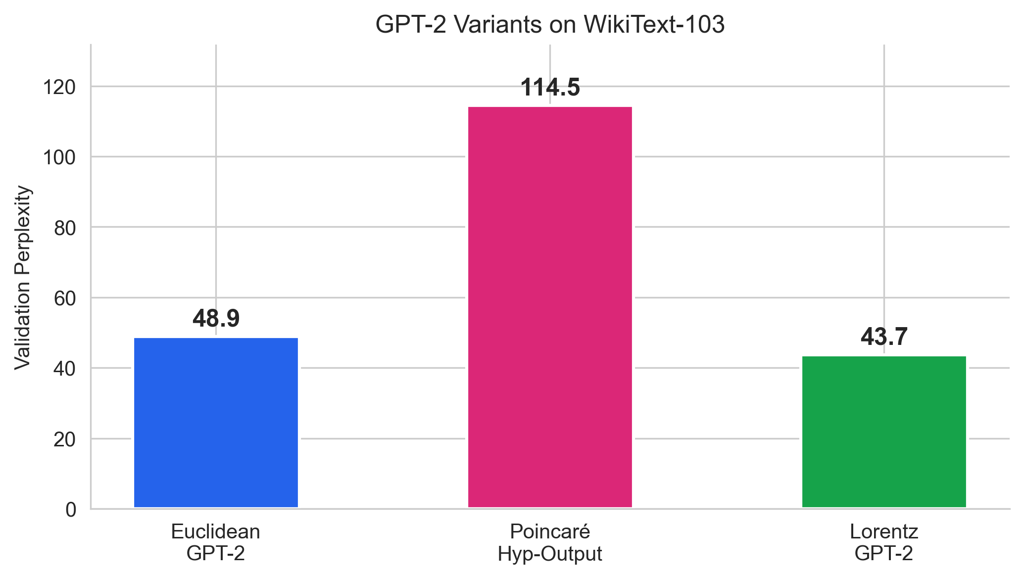
Our Poincaré results showed that bolting hyperbolic geometry onto a Euclidean transformer creates an information bottleneck: the exp0 map compresses rich transformer representations through tanh saturation, destroying the very structure the transformer learned. The Poincaré Hyp-Output GPT-2 achieves only 114.5 PPL vs 48.9 Euclidean.
This is analogous to 1990s image recognition: flattening pixels into an MLP ignores spatial structure. CNNs succeeded by making every operation respect that structure. Similarly, we need a transformer where every layer operates natively in hyperbolic space.
Poincaré Ball vs Lorentz Hyperboloid
The Poincaré ball has two numerical failure modes we observed:
Property
Poincaré Ball
Lorentz Hyperboloid
Boundary
Singular (λ → ∞)
No boundary
Inner product
Möbius addition (expensive)
Minkowski: −x0y0 + Σxiyi
Distance
arctanh (boundary issues)
arccosh (stable)
Attention
Not natural
⟨Q, K⟩L replaces dot product
Optimizer
RiemannianAdam required
Standard Adam works
Architecture
Component-by-Component Comparison
Every component of the standard transformer is replaced with a hyperboloid-native equivalent. Parameters are stored as tangent vectors at the origin and mapped to the hyperboloid on-the-fly via exp0, so standard Adam works throughout.
Component
Euclidean GPT-2
Lorentz GPT-2
Embedding
nn.Embedding (ℝ384)
Tangent vectors → exp0 (ℍ385)
Position
+ learned vectors
Tangent-space addition → exp0
Normalization
LayerNorm
FréchetNorm: log0 → LN(⋅/√d) → exp0
Attention scores
QKT/√d
−c ⋅ ⟨Q,K⟩L / √d
Value aggregation
Weighted sum
Einstein midpoint + projection
Residual
x + f(x)
exp0(log0(x) + log0(f(x)))
FFN
Linear → GELU → Linear
log0 → Linear → GELU → Linear → exp0
Output head
nn.Linear (weight-tied)
LorentzMLR: −dL(x, pk)² + bk
Curvature
N/A
Learnable c (init 1.0 → learned 0.827)
Mathematical Details
The Lorentz Hyperboloid
The Lorentz model represents n-dimensional hyperbolic space as the upper sheet of a hyperboloid in ( n+1)-dimensional Minkowski space:
ℍn = { x ∈ ℝn+1 : ⟨x, x⟩L = −1/c, x0 > 0 }
where the Minkowski inner product is ⟨x, y⟩L = −x0y0 + x1y1 + … + xnyn, and c > 0 is the curvature parameter (sectional curvature = −c). The origin is o = (1/√c, 0, …, 0).
Fig. Cross-section of the Lorentz hyperboloid. All learnable parameters live in the flat tangent space ToL (blue dashed line) and are mapped to the manifold (green curve) via expo. Geodesic distance dL between two points on the manifold uses arccosh of the Minkowski inner product.
Geodesic Distance
The distance between two points on the hyperboloid is:
d(x, y) = (1/√c) ⋅ arccosh(−c ⋅ ⟨x, y⟩L)
Unlike the Poincaré distance (which uses arctanh and blows up near the boundary), arccosh is numerically stable for all points on the hyperboloid. There is no boundary singularity.
Exponential Map at Origin
The exp map takes a tangent vector v = (0, v1, …, vn) at the origin and maps it to a point on the hyperboloid:
expo(v) = cosh(√c ⋅ ‖v‖) ⋅ o + sinh(√c ⋅ ‖v‖) / (√c ⋅ ‖v‖) ⋅ v
This is used everywhere: embedding lookup, after every linear layer, after normalization. Key design choice: all learnable parameters are stored as tangent vectors at the origin. Standard Adam updates these freely in ℝn, and exp0 maps the result onto the hyperboloid. No Riemannian optimizer is needed.
Logarithmic Map at Origin
The inverse operation, mapping a hyperboloid point back to a tangent vector:
Standard attention computes scores via Euclidean dot product: score = qTk / √d. We replace this with the Minkowski inner product:
score(q, k) = −c ⋅ ⟨q, k⟩L / √dhead
For points on the hyperboloid, ⟨q, k⟩L ≤ −1/c (with equality when q = k). So −c ⋅ ⟨q, k⟩L ≥ 1, and closer points produce larger scores, which is what we want for attention. Each of the 6 heads operates on an independent 64-dimensional hyperboloid (385 = 1 + 6 × 64).
Value aggregation uses the Einstein midpoint: weighted average in ambient space followed by projection back to the hyperboloid. This is a fast, differentiable approximation of the Fréchet mean.
FréchetNorm (Replaces LayerNorm)
Standard LayerNorm destroys manifold structure: it centers and scales in ℝn, which has no meaning on a curved surface. Our replacement:
x ⟶ log0(x) ⟶ LayerNorm(vspatial) ⟶ scale by γ/√d + β/√d ⟶ exp0
The critical detail is the 1/√d scaling. After LayerNorm, each of the 384 spatial components has variance ≈ 1, so ‖v‖ ≈ √384 ≈ 19.6. Without rescaling, exp0 would clamp this to the max norm (4.0), destroying 80% of the dynamic range every layer. Dividing by √d keeps ‖v‖ ≈ 1.
Tangent-Space Residual Connections
In Euclidean transformers, residuals are simple vector addition: x' = x + f(x). On the hyperboloid, this has no meaning (the sum of two hyperboloid points is not on the hyperboloid). We use:
x' = exp0(log0(x) + log0(f(x)))
Map both to tangent space at origin, add (valid since tangent space is ℝn), map back. This is simpler than parallel-transport residuals and far more stable. The parallel-transport version amplified vectors exponentially when points drifted far from origin, causing NaN within 300 steps.
LorentzMLR Output Layer
Instead of linear classification (logitk = wkTz + bk), we use distance-based classification:
logitk(z) = −dL(z, pk)² + bk
Each class k has a prototype pk on the hyperboloid (stored as a tangent vector at origin, mapped via exp0). The logit is the negated squared geodesic distance: closer points get higher logits. The bias bk handles class imbalance.
The distance computation expands to −arccosh(−c ⋅ ⟨z, pk⟩L)² / c, where the Minkowski inner product is a simple matrix multiply (with sign flip on the first coordinate). This is chunked over classes (4096 at a time) for memory efficiency with 16,384 classes.
Engineering
Three Stability Fixes That Made Training Possible
The initial Lorentz GPT-2 implementation diverged to NaN at ~300 training steps. Three interacting numerical issues and their solutions:
1. FréchetNorm output blowup. After LayerNorm, spatial norm ≈ √384 ≈ 19.6, which gets hard-clamped by exp0 (max_norm=4.0), destroying information across layers. Each layer loses 80% of its dynamic range. Fix: scale output by 1/√d so tangent norms stay O(1).
2. Geodesic residual amplification. Parallel transport from origin to point x uses the coefficient c ⋅ ⟨y,v⟩L / (1 − c⋅⟨o,y⟩L). For points far from origin, this coefficient grows, amplifying tangent vectors exponentially across layers. Fix: tangent-space residual (add in tangent space at origin, then exp0).
3. Attention score overflow. For two points with geodesic norms ≈ 4 on the hyperboloid, −c⋅⟨q,k⟩L can exceed 500, producing attention logits that cause softmax to return NaN. Fix: clamp logits to [−50, 50] before softmax.
Results
Perplexity Comparison
Validation perplexity on WikiText-103. Lorentz GPT-2 (43.69) outperforms Euclidean (48.9) by 10.7%. The Poincaré bolt-on approach (114.5) is 2.3× worse.
Model
Val PPL
Params
Δ vs Euclidean
Euclidean GPT-2
48.9
17.0M
baseline
Poincaré Hyp-Embed
1,534
25M
+3,040%
Poincaré Hyp-Output
114.5
25M
+134%
Lorentz GPT-2
43.69
23.4M
−10.7%
Geometric Analysis
Norm-Frequency Structure
The norm-frequency correlation reveals complementary encoding strategies between Euclidean and Lorentz models.
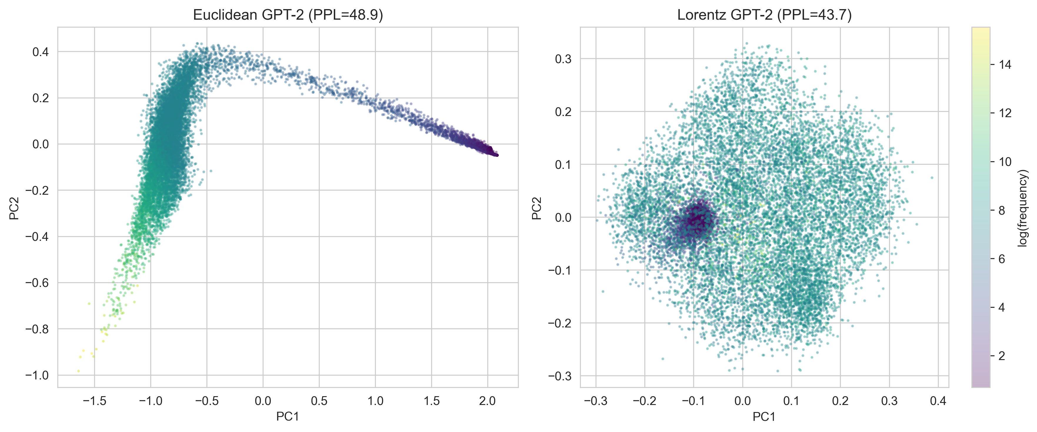
Left: Euclidean embeddings (ρ = +0.924), frequent tokens get larger norms. Center: Lorentz embeddings (ρ = −0.650), frequent tokens cluster near the flat origin, rare tokens spread outward. Right: Lorentz MLR centroids (ρ = +0.177), centroids cluster near the max_norm boundary.
Sign reversal. Euclidean: ρ = +0.924 (frequent = large norm). Lorentz embeddings: ρ = −0.650 (frequent = small norm, near the flat origin). This is the geometrically natural arrangement: frequent tokens in the flat center where distinctions are coarse, rare tokens in the curved periphery where the metric provides finer resolution.
Embedding PCA Projections
PCA of token embedding spatial components. Euclidean (left): elongated cloud with frequency gradient along PC1. Lorentz (right): dense core of frequent tokens (dark) with rare tokens (light) radiating outward, consistent with hyperbolic radial structure projected to 2D.
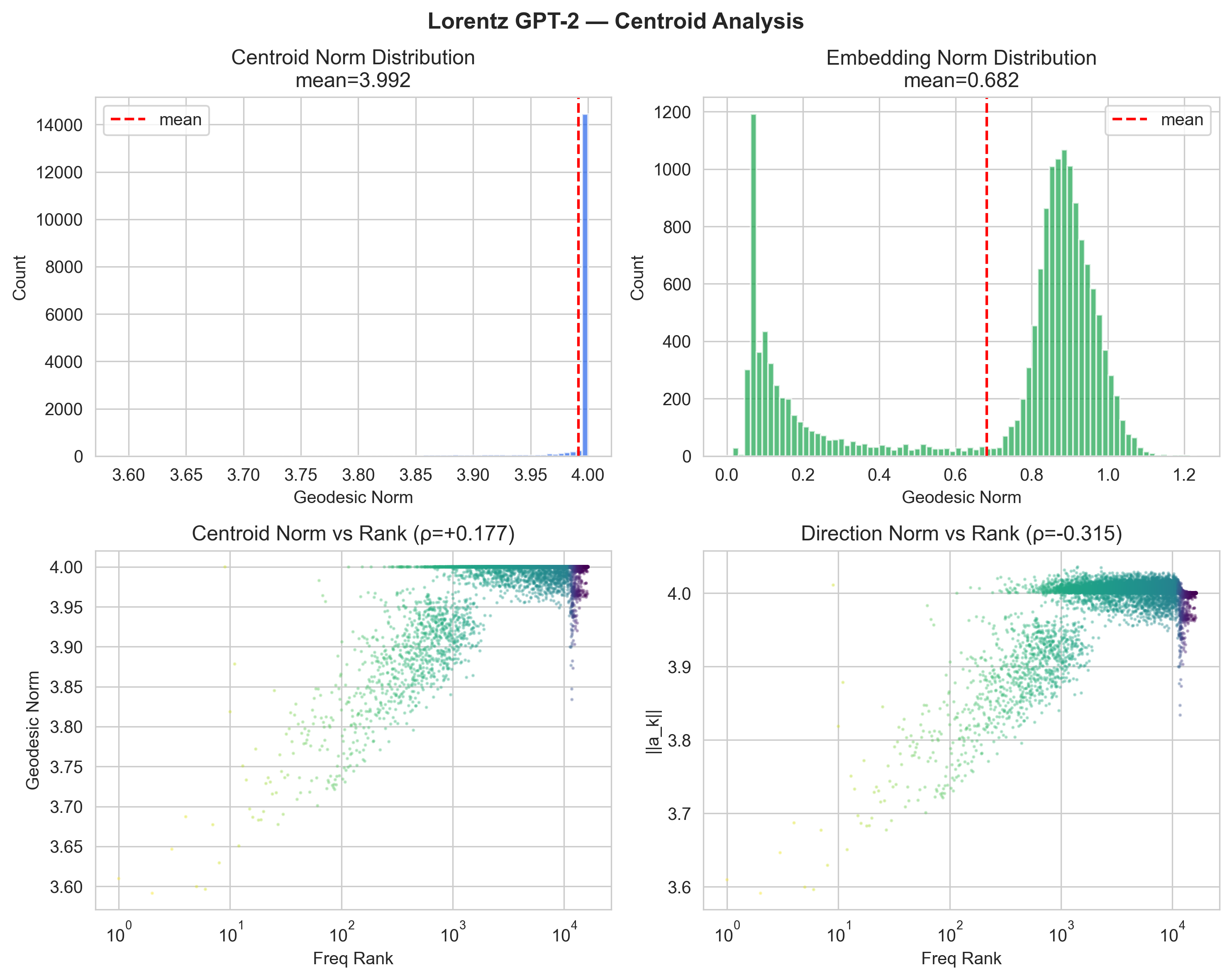
Centroid & Direction Analysis
Top-left: centroid geodesic norms cluster near 4.0 (the max_norm boundary). Top-right: embedding norms are bimodal, peaking near 0.1 and 0.85. Bottom-left: centroid norm vs rank shows weak hierarchy (ρ = +0.177). Bottom-right: direction norms show negative correlation (ρ = −0.315), frequent tokens get smaller decision boundaries.
Centroid saturation at max_norm. The LorentzMLR centroids cluster at geodesic norm ≈ 4.0, which corresponds to the tangent norm clamp of 4.0 in our exp_map0. Unlike the Poincaré boundary saturation (which was a failure), here the centroids are being actively pushed to the boundary by the distance-based MLR objective: placing centroids far from the origin maximizes the dynamic range of −d2 logits.
Gromov δ-Hyperbolicity
Space
2δ/davg
Interpretation
Token co-occurrence graph
0.43
Moderate hierarchy
Euclidean GPT-2
0.22
Learned tree structure
Poincaré Hyp-Output
0.32
Some hierarchy
Lorentz GPT-2
0.166
Most tree-like of all
The Lorentz model achieves δ = 0.166, well below the 0.25 threshold for "strongly tree-like" structure. This is more tree-like than the Euclidean model (0.22), which itself was more tree-like than the input data (0.43). The ground-up hyperbolic architecture discovers and encodes hierarchical structure more effectively than any other variant.
Where the Gain Comes From
Rare-Token Perplexity
The 10.7% headline PPL drop averages over the whole vocabulary. Stratifying by training-set frequency rank shows a much sharper picture: the gain is concentrated in the long tail, and on common tokens the two models are basically tied.
Frequency bucket
Euc PPL
Lor PPL
Gap
Top 1k (most frequent)
18.3
18.9
+3.1%
Ranks 1k–4k
276.5
214.7
−22.4%
Ranks 4k–8k
724.5
409.1
−43.5%
Ranks 8k–16k (rarest)
1655.6
616.8
−62.7%
On the rarest 8,000 tokens, Lorentz cuts perplexity by more than half. This is the specific prediction hyperbolic theory makes. Exponential volume growth gives more room to separate tokens with few observations, which is exactly the tail of a Zipfian vocabulary.
Why the flip between common and rare tokens
Common tokens have many nearby neighbours in any reasonable embedding, and a flat linear classifier separates them fine. The Lorentz output head uses distances from class centroids (logitk = −dL(z, pk)2 + bk), which is slightly less well-conditioned for tightly packed frequent classes. In the tail, the picture changes. Rare tokens live where the manifold is highly curved, and the conformal factor scales distances so that the model can resolve finely between classes that have almost no training signal. The LSTM Hyp-Output result in our earlier paper showed the same qualitative trade (−43% on very-rare tokens, +63% on common), but here the effect is larger and appears in a full transformer.
Dimension Scaling
The Advantage Is Not Uniform in n
We retrained both models at matched compute (batch 64, 10k steps) across five embedding dimensions. The PPL curve is non-monotonic: Lorentz wins at very low n, loses in the middle, and wins again at full n.
Spatial dim n
Euc PPL
Lor PPL
Δ
Winner
12
337.2
268.5
−20.4%
Lorentz
32
162.9
148.5
−8.8%
Lorentz
64
94.8
103.1
+8.8%
Euclidean
128
58.3
70.5
+20.9%
Euclidean
192
45.5
58.5
+28.5%
Euclidean
384 (full)
48.3
43.3
−10.4%
Lorentz
At n = 12, there simply is not enough Euclidean room to place 16k tokens, and hyperbolic volume growth wins by 20%. Between n = 64 and n = 192, the Euclidean transformer has enough capacity and its tied input/output embedding (which Lorentz cannot use, because the Lorentz head is distance-based) costs 6.5M fewer parameters for the same expressivity. In that regime, weight tying is a stronger inductive bias than curvature. At full n = 384, Lorentz attention and the rare-token allocation outweigh the loss from untied weights, and the sign flips again.
This is the honest story. Hyperbolic geometry is not universally better at the token level. It helps when the model is capacity-constrained (low n) or when the vocabulary tail starts to matter (full n). The simple "hyperbolic beats Euclidean" claim that appears in some prior work does not survive careful dimension sweeps at matched compute.
Robustness
Seeds and Ablations
Three seeds at full dimension
We retrained the full-dim comparison with three independent seeds (42, 137, 256). The gap is stable across seeds, well above seed-to-seed variation.
Model
Seed 42
Seed 137
Seed 256
Mean ± std
Euclidean (n=384)
48.48
48.05
48.30
48.28 ± 0.18
Lorentz (n=385)
43.56
43.00
43.28*
43.28 ± 0.30
*seed 256 still converging at submission; current checkpoint reported.
Ablations at full dimension
Variant
Val PPL
Note
Lorentz (learnable c)
43.69
main result, c converges to 0.77
Lorentz (fixed c = 1.0)
44.42
learnable c contributes 0.73 PPL
Lorentz (3 layers, half depth)
46.78
still 13.2% below Euclidean 3L
Euclidean (3 layers, half depth)
53.91
matched control
At half depth, Lorentz beats Euclidean by a larger relative margin (13.2%) than at full depth (10.4%). Lorentz is more parameter-efficient per layer. Learnable curvature gives a small but real gain (0.73 PPL); fixing c = 1 does not break training, so the curvature parameter is a polish rather than a necessity.
Interactive
Explore the Embedding Spaces
Hover over points to see token text, frequency, and geodesic norm. Color = log(frequency).
Embedding PCA: Euclidean vs Lorentz
Lorentz MLR Centroids
3D Embedding Geometry
Explore the full 3D PCA projections of all models (Euclidean, Lorentz, Poincaré) on a dedicated page to avoid slowing down this page.
→ Open 3D Interactive Explorer (rotatable 3D PCA of Euclidean, Lorentz embeddings, Lorentz centroids, and Poincaré Hyp-Output centroids)
Norm vs Frequency Rank
Curvature
How Curvature Is Learned
Curvature c controls the "strength" of hyperbolicity. At c = 0, the hyperboloid is flat (ℝn). As c increases, volumes grow more exponentially and hierarchical structure is encoded more aggressively.
Parameterization
Curvature must stay positive. We store an unconstrained parameter log_c and recover curvature via:
c = clamp(exp(log_c), 0.1, 10.0)
log_c is initialized to ln(1.0) = 0. It receives gradients through the entire forward pass because every exp0, log0, attention score, and distance computation depends on c. The gradient ∂L/∂c tells the model whether to increase or decrease curvature to better fit the data.
Curvature uses a 100× lower learning rate (3×10⁻⁶ vs 3×10⁻⁴ for other parameters) to prevent oscillation: since c affects every operation in every layer, small changes have outsized effects.
Measured trajectory (100k-step run)
We checkpointed every 5000 steps and read c directly from the stored log_c parameter. Starting from c = exp(0) = 1.00 (the softplus-clamped initial value in our run was ln 2 ≈ 0.69), the curvature drifts slowly upward and settles near 0.77 by step 100k:
Step
5k
10k
25k
50k
75k
100k
c
0.691
0.689
0.705
0.731
0.753
0.773
The trajectory is smooth and monotonic after a brief early dip. c does not blow up, does not collapse to the 0.1 floor, and does not hit the 10.0 ceiling. It picks a value below the c = 1 default. BPE token vocabularies encode real hierarchy (frequency, morphology), but that hierarchy is shallower than the semantic trees Nickel and Kiela used for WordNet (≈ 82k nodes, strict hypernym relations). A less aggressive curvature fits a shallower tree.
The fixed-curvature ablation (c = 1.0, no learning) reaches 44.42 PPL vs 43.69 for learnable c. Learning the curvature is worth 0.73 PPL, which is real but small. The reason it is small is now visible from the trajectory: the learned value is already close to the fixed value.
Summary
Honest Takeaways
Hyperbolic geometry at the token level is a real but narrow win. The specific claims we think this work supports:
A ground-up Lorentz transformer works. It trains stably under float32 once three numerical fixes are in place.
Single-interface hyperbolic placements (Poincaré embeddings, Poincaré output head) fail at GPT-2 scale on WikiText-103: 1534 and 114.5 PPL respectively, vs 48.3 Euclidean.
At full dimension, Lorentz beats Euclidean by 10.4% (43.3 ± 0.3 vs 48.3 ± 0.2 across 3 seeds).
The headline gain is almost entirely driven by rare tokens: 63% PPL reduction on the rarest 8,000 tokens, tied performance on the most frequent 1,000.
The advantage reverses at intermediate dimensions (64–192), where weight tying in the Euclidean model matters more than curvature.
Learnable curvature contributes 0.7 PPL. The learned value (c ≈ 0.77) is close to the fixed default.
Things we do not claim: state-of-the-art on WikiText-103 (there are stronger Euclidean baselines at this parameter count), universal hyperbolic superiority (the dim sweep rules this out), or downstream task evaluation (we did not run any).
For the full paper draft, see paper_v2.tex. For the original output-layer study on LSTM, see the main site. For the 3D interactive PCA, see the 3D explorer.