Analysis Overview
This page collects all experimental results, figures, and structural diagnostics from our two-phase study. Phase 1 places embeddings directly in the Poincare ball; Phase 2 keeps embeddings Euclidean and applies geometry only at the output layer. The Poincare GloVe section provides the reference picture of what successful hyperbolic embeddings look like.
Phase 1 - Full Hyperbolic Embedding
Following Nickel & Kiela (2017): embeddings live in the Poincare ball,
optimized via RiemannianAdam with a 500-step burn-in phase. Embeddings are
mapped to tangent space before the LSTM via logmap0.
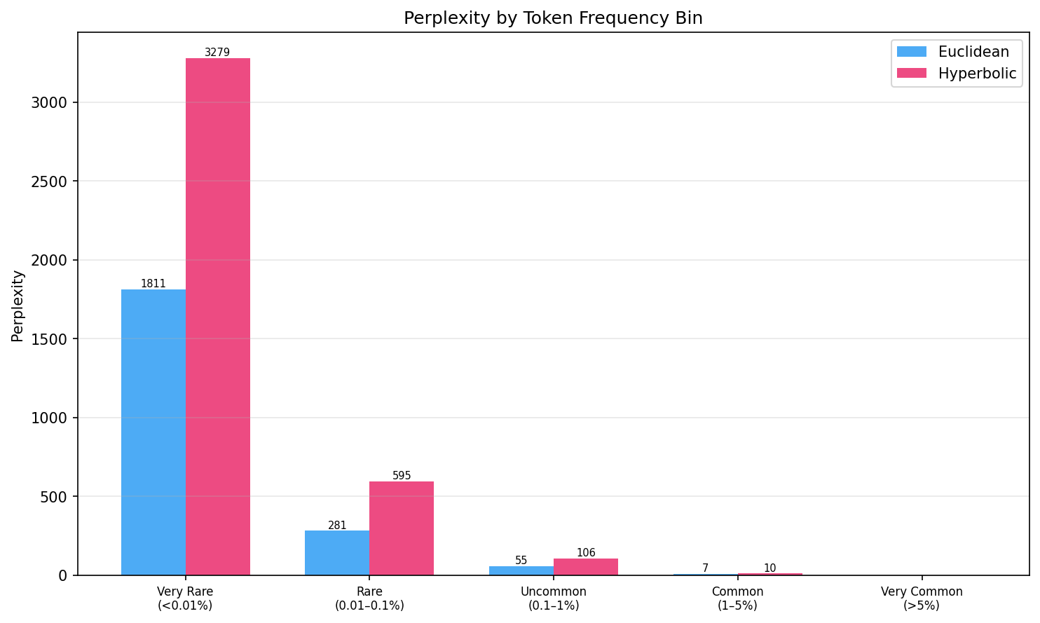
Perplexity by Token Frequency Bin
We stratify validation perplexity by token frequency to test the hypothesis that hyperbolic geometry helps with rare tokens. If the curved space encoded a frequency hierarchy, rare tokens near the ball boundary should have better representations.
Raw Numbers
Blue = Euclidean, Pink = Hyperbolic. Bars scaled relative to max (3279).
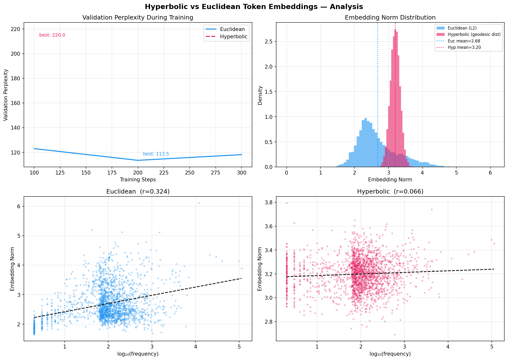
Embedding Norm Diagnosis
The crucial diagnostic: do embedding norms correlate with token frequency? In Nickel & Kiela's framework, a well-trained hyperbolic embedding places general tokens near the origin (small norm) and specific rare tokens near the boundary (large norm).
Phase 2 - Output-Layer Geometry
Motivated by Moreira et al. (2023): embeddings and LSTM remain fully Euclidean; only the output classification layer uses geometry. This avoids boundary saturation while still testing whether hyperbolic distance structure aids classification. All three variants (Euclidean, Hyperbolic, Spherical) use identical Adam optimizers -- no manifold learning rates or burn-in phases.
Phase 2 Perplexity Results
| Run ID | Type | Emb Dim | Hidden | Dropout | Steps | Best Val PPL | Train PPL |
|---|---|---|---|---|---|---|---|
| run-20260308_132126 | euclidean | 256 | 256 | 0.2 | 15 000 | 120.1 | 88.6 |
| run-20260308_135230 | hyperbolic | 256 | 256 | 0.2 | 15 000 | 117.4 | 57.7 |
| run-20260308_132127 | spherical | 256 | 256 | 0.2 | 15 000 | 121.7 | 76.6 |
Phase 2 Architecture Detail
| Component | Euclidean | Hyperbolic | Spherical |
|---|---|---|---|
| Embedding | R^256 | R^256 | R^256 |
| LSTM (1 layer) | R^256 | R^256 | R^256 |
| Projection | Identity | expmap0 to Poincare ball | L2 normalize to sphere |
| Classifier | Linear (8192) | HyperbolicMLR (Ganea 2018) | Linear on sphere |
| Optimizer | Adam 1e-3 | Adam 1e-3 | Adam 1e-3 |
Why Phase 1 Fails: Boundary Saturation
Moreira et al. (2023) give a precise theoretical explanation for the Phase 1 failure, and our diagnostics confirm it exactly.
The Theoretical Argument
In d-dimensional hyperbolic space, the ratio of ball volume to ball surface area is bounded by r/d. As d grows this ratio approaches 0, exactly as in Euclidean space. All volume concentrates at the boundary. Given that cross-entropy loss is unbounded below as embeddings approach the unit ball boundary, the optimizer follows the gradient to the boundary.
Once all embeddings lie at radius r_eff = (1-epsilon)/sqrt(-k), the Poincare distance between any two points u, v with ||u||=||v||=r_eff reduces to a function of the angle between them only. The space is then isometric to a Euclidean sphere -- the radial hierarchy-encoding property is lost entirely.
# From our diagnostics (Phase 1, 15k steps, dim=256):
euclidean_mean_norm  = 2.68   # broad distribution
hyperbolic_mean_norm = 3.20   # saturated at boundary
hyperbolic_std_norm  = 0.05   # extremely tight clustering

# Poincare ball boundary = 1.0 (normalized), but with curvature k=1
# r_eff ~ (1-epsilon) / sqrt(k) ~ 1.0 in Poincare parameterization
# Our embedding norms show saturation in geoopt's non-unit-ball parameterization

# Norm-frequency correlation:
r_euclidean = 0.335   # clear hierarchical structure
r_hyperbolic = 0.045  # no structure
Why Phase 2 Avoids This
Phase 2 never places the embedding table in the Poincare ball. The LSTM hidden state (a 256-dim Euclidean vector) is projected to the ball only at the final classification step, where it is used as a query point for hyperbolic softmax. There is no pressure for this single projection to saturate, since the hidden state itself is regularized by the language modeling task and dropout.
Reference: Poincare GloVe Analysis
From Tifrea et al. (2019). These plots show what successful hyperbolic embeddings look like on full-word vocabulary (190k words, 20D). This is the gold standard our BPE token embeddings should eventually approach.
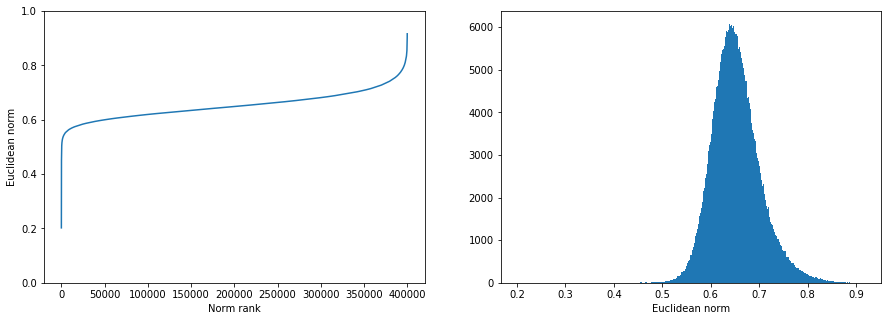
Norm vs Frequency Rank - Full Words
Key statistics from the notebook: Spearman r(norm, frequency) = -0.69 for Poincare target vectors, -0.61 for standard GloVe -- a measurable but modest improvement from hyperbolic geometry. Hyperbolic mean norm 0.653, std 0.050 (compared to our token embeddings at 3.2 +/- 0.05 in a different Poincare ball parameterization).
Distance Structure - Poincare vs Euclidean
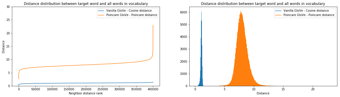
Average Relative Contrast: Poincare 4.46 (top 100) / 2.03 (rest) vs GloVe 16.1 (top 100) / 2.32 (rest). Interestingly GloVe has higher ARC for top-100 frequent words in this metric -- hyperbolic geometry spreads the semantic space but at the cost of anchor stability for the most common words.
Nearest Neighbor Quality (from notebook)
| Word | Poincare GloVe Nearest Neighbors |
|---|---|
| dance | dancing, dances, music, singing, musical, performing, hip-hop, pop, folk, dancers |
| sixties | seventies, eighties, nineties, 60s, 70's, 60's, 1960's, 80's, 90's, 70s |
| daughter | son, wife, mother, sister, father, husband, brother, daughters, sons, grandmother |
Nearest neighbors in Poincare distance are semantically coherent and capture analogical structure. This is what well-trained hyperbolic embeddings can produce. At the subword BPE level, analogous quality would mean tokens like -ing clustering near general morphological roots, with rare compositional tokens near the boundary.
Center vs Border of the Ball
| Location | Sample Words (190k vocab Poincare GloVe) |
|---|---|
| Near center (small norm) general, abstract |
alola, arecoideae, gnetophytes, chennselaig, wesleys, duckwater -- very rare, specific named entities |
| Near border (large norm) specific, frequent |
singles, race, road, hockey, i, starring, player, income, rural, yards -- common topical words |
Interactive: Cherry-picked Semantic Hierarchies
From Tifrea et al. (2019). The Poincare GloVe model uses 20-dimensional embeddings decomposed into 10 separate 2D Poincare disks (one subplot per embedding slot). Each disk shows 6 semantic categories -- presidents, mathematics terms, numbers, chemistry, sports figures, countries -- each as a colored cluster. Hover over points to see word labels. Use the Plotly toolbar to zoom, pan, or export.
Context vectors for 180k-word vocabulary. All 10 disks share the same [-1, 1] x [-1, 1] range to keep the Poincare ball boundary visible.
Poincare GloVe MIX model (20D, 10 x 2D Poincare disks, dist-sq objective, 180k vocab). Each subplot is one 2D Poincare disk. The boundary at radius 1 is the Poincare ball limit.
All Runs
Complete table of all wandb runs with metrics and configurations.
| Run ID (timestamp) | Phase | Type | Emb Dim | Hidden | Dropout | Steps | Best Val PPL | Train PPL |
|---|---|---|---|---|---|---|---|---|
| 20260307_133535 | 1 | hyperbolic | 256 | 512 | 0 | 400 | 698.3 | 656.9 |
| 20260307_133536 | 1 | hyperbolic | 256 | 512 | 0 | 200 | 984.3 | 656.6 |
| 20260307_134408 | 1 | euclidean | 256 | 512 | 0 | 240 | 593.4 | 549.0 |
| 20260307_135727 | 1 | euclidean | 256 | 512 | 0 | 5 000 | 121.8 | 71.7 |
| 20260307_135842 | 1 | hyperbolic | 256 | 512 | 0 | 5 000 | 186.7 | 114.4 |
| 20260307_235654 | 1 | euclidean | 256 | 512 | 0.2 | 5 000 | 124.5 | 62.2 |
| 20260307_235900 | 1 | hyperbolic | 256 | 512 | 0.2 | 5 000 | 203.3 | 138.8 |
| 20260308_010154 | 1 | hyperbolic | 256 | 512 | 0.2 | 2 360 | 354.2 | 282.2 |
| 20260308_021526 | 1 | hyperbolic | 256 | 512 | 0.2 | 15 000 | 174.0 | 76.2 |
| 20260308_021528 | 1 | euclidean | 256 | 512 | 0.2 | 15 000 | 113.5 | 36.3 |
| 20260308_132126 | 2 | euclidean | 256 | 256 | 0.2 | 15 000 | 120.1 | 88.6 |
| 20260308_135230 | 2 | hyperbolic | 256 | 256 | 0.2 | 15 000 | 117.4 | 57.7 |
| 20260308_132127 | 2 | spherical | 256 | 256 | 0.2 | 15 000 | 121.7 | 76.6 |
Open Questions and Future Work
1. Is the Token Co-occurrence Graph Hyperbolic?
Tifrea et al. measure the Gromov delta-hyperbolicity of word co-occurrence graphs and find 2*delta_avg/d_avg ratios as low as 0.0034, confirming that word co-occurrence data is genuinely tree-like. This measurement has not been performed for BPE subword tokens. BPE tokens are defined by frequency-based compression, not semantic content, and their co-occurrence structure may differ fundamentally from full-word graphs.
2. Do Phase 2 Embeddings Show Radial Structure?
The Phase 2 models have not yet been subjected to the norm-vs-frequency diagnostic. Since embeddings remain Euclidean, the interesting question is whether the LSTM hidden state, when projected to the Poincare ball, develops radial structure tied to the frequency of the next token being predicted.
3. Overfitting in Phase 2 Hyperbolic
Hyperbolic MLR train PPL (57.7) vs val PPL (117.4) shows a larger train/val gap than Euclidean (88.6 / 120.1). The hyperbolic output layer may have more capacity due to the richer distance structure, but this capacity is not yet being regularized effectively. Investigating dropout rates and weight decay specifically for the hyperbolic output parameters is the immediate next experiment.
4. Low-Dimension Regime
Theory predicts hyperbolic space should show the clearest advantages at low embedding dimensions (e.g., dim=8 or 16), where Euclidean space genuinely struggles to represent hierarchical structure. Our current experiments all use dim=256. Running a dimension sweep (8, 16, 32, 64, 128, 256) with Phase 2 architecture is the most direct test of the theoretical prediction.